你们有用手机拍照吗?我偶尔会拍。自从智能手机问世以来,已经过了一段时间,手机的相机技术也有了很大的进步。现在拍出的照片之美,甚至让我觉得可能不再需要单反相机了。(当然,在黑暗环境下,效果还是有很大差距的……)我想对手机中使用的图像传感器的性能进行一些分析!!
使用在 iPhone 中的图像传感器。
我手中的智能手机是 iPhone 12,所以我将分析 iPhone 12 中使用的图像传感器。首先,我会调查 iPhone 12 中使用的图像传感器。经过一番搜索,我找到了一个网站,根据那里的信息,iPhone 12 的广角相机使用的是 Sony 生产的 IMX503 图像传感器。我想知道 IMX503 是什么样的传感器,所以我进行了调查,但无论怎么查,都找不到数据手册。我想这可能不是市售产品,而是专为苹果开发的传感器。
图像传感器的测量方法。
那么,进入正题,关于图像传感器的分析方法。这次我们将检查传感器的输出响应和噪声性能。准备的材料如下:
- iPhone(可获取 Raw 格式的相机)
- ND 滤镜 15 段
- 平坦的光源
- 黑暗空间
- 电脑(Python)
进行图像传感器分析时,需要获取 Raw 图像。iPhone 用户通常无法通过普通相机获取 Raw 图像。如果你想在 iPhone 上获取 Raw 图像,可以试试这款应用(简单 Raw 相机)。Raw 格式为 DNG 文件。
光源尽量选择平坦的。如果有积分球的朋友可以使用积分球。如果没有平坦的光源,可以将电脑显示器调到最大亮度,并设置为全白色。
ND 滤镜当然是用来降低光量的。如果没有 ND 滤镜,可以尝试使用快门速度来调整光量。(不过,这样可能会改变噪声特性。)
这里最重要的是,测量必须在完全黑暗的空间中进行。这是为了确保在暗区附近的线性度不会受到影响。
接下来是实际的测量方法。
- 固定光源和相机的位置(确保 ND 滤镜全部能进入)。
- 将光源调亮至相机接近饱和的状态。如果光源亮度不足以导致饱和,可以尝试延长快门速度。
- 开始拍摄光源。从最亮的状态开始,每次将光量减少一半,重复拍摄。减少光量的方法可以是插入 ND 滤镜或调整快门速度。
- 拍摄完从饱和到足够暗的状态后,数据收集完成。
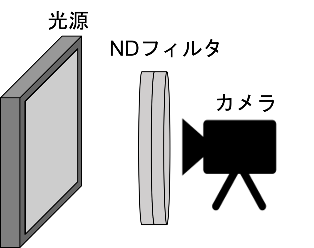
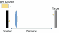
注意事项是,保持光源和相机的距离不变。如果将光源移得更远,光线自然会变暗。以下是配置的示意图:
Raw 数据的分析。
首先,通过 iPhone 或单反相机获取的 Raw 图像通常是各家公司特有的格式,因此在开始分析之前,需要将其转换为通用 Raw 格式。
我们将对获取的数据进行分析。这次我将使用 Python 来进行分析。此次使用的库是:
import numpy as np
import matplotlib.pyplot as plt
import math
这是代码整体的流程。虽然有点长,但请耐心阅读到最后。
- Raw 图像读取设置
- 设置用于图像处理的 Numpy 数组
- 处理多张 Raw 图像的设置
- 减去暗电流(此次设定为 528)
- 计算信号、噪声和信噪比
- 显示图表
以下是实际的代码:
import numpy as np
import matplotlib.pyplot as plt
import math

#***********************************
#1. Image Settings
#***********************************
width = 4032
height = 3024
width_roi = 100
height_roi = 100
image_num = 15
bit = 12
dark = 528

half_width = int(width / 2)
half_height = int(height / 2)
half_width_roi = int(width_roi / 2)
half_height_roi = int(height_roi / 2)

#***********************************
#2. Array Creation
#***********************************
img_roi = np.empty((height_roi, width_roi), dtype=np.uint16)  # Empty array
img_s = np.empty((4, image_num), dtype=np.float32)
img_n = np.empty((4, image_num), dtype=np.float32)
img_sn = np.empty((4, image_num), dtype=np.float32)
rgb = np.array(range(4))  # For RGB distribution
rgb_det = rgb.reshape((2, 2))  # For RGB distribution
img_roi_r = np.empty((half_height_roi, half_width_roi), dtype=np.uint16)
img_roi_gr = np.empty((half_height_roi, half_width_roi), dtype=np.uint16)
img_roi_gb = np.empty((half_height_roi, half_width_roi), dtype=np.uint16)
img_roi_b = np.empty((half_height_roi, half_width_roi), dtype=np.uint16)
x_axis = np.empty((1, image_num), dtype=np.uint16)

#***********************************
#3. Processing Multiple Raw Images
#***********************************
for i in range(image_num):
    x_axis[0][i] = 2 ** i
    rawpath = "DNG_4032x3024_dark=528_12bit_lin" + str(i) + ".raw"  # Raw image name
    #***********************************
    # Open raw image
    #***********************************
    fd = open(rawpath, 'rb')
    f = np.fromfile(fd, dtype=np.uint16, count=height * width)
    img = f.reshape((height, width))
    fd.close()

    #***********************************
    # Extract ROI
    #***********************************
    width_roi_start = int((width - width_roi) / 2)
    height_roi_start = int((height - height_roi) / 2)
    for x in range(width_roi_start, width_roi_start + width_roi):
        for y in range(height_roi_start, height_roi_start + height_roi):
            img_roi[y - height_roi_start][x - width_roi_start] = img[y][x]

    #***********************************
    # Dark subtraction
    #***********************************
    for x in range(width_roi):
        for y in range(height_roi):
            if img_roi[y][x] > dark:
                img_roi[y][x] = img_roi[y][x] - dark
            elif img_roi[y][x] <= dark:
                img_roi[y][x] = 0

    #***********************************
    # SN Calculation
    #***********************************
    for x in range(width_roi):
        for y in range(height_roi):
            color = rgb_det[y % 2][x % 2]
            if color == 0:  # R
                y_r = int(y / 2)
                x_r = int(x / 2)
                img_roi_r[y_r][x_r] = img_roi[y][x]
            elif color == 1:  # Gr
                y_gr = int(y / 2)
                x_gr = int((x - 1) / 2)
                img_roi_gr[y_gr][x_gr] = img_roi[y][x]
            elif color == 2:  # Gb
                y_gb = int((y - 1) / 2)
                x_gb = int(x / 2)
                img_roi_gb[y_gb][x_gb] = img_roi[y][x]
            else:  # B
                y_gb = int((y - 1) / 2)
                x_gb = int((x - 1) / 2)
                img_roi_b[y_gb][x_gb] = img_roi[y][x]

    # Signal
    img_s[0][i] = np.mean(img_roi_r)
    img_s[1][i] = np.mean(img_roi_gr)
    img_s[2][i] = np.mean(img_roi_gb)
    img_s[3][i] = np.mean(img_roi_b)

    # Noise
    img_n[0][i] = np.std(img_roi_r)
    img_n[1][i] = np.std(img_roi_gr)
    img_n[2][i] = np.std(img_roi_gb)
    img_n[3][i] = np.std(img_roi_b)

    # SNR
    img_sn[0][i] = 20 * (math.log10(img_s[0][i] / img_n[0][i]))
    img_sn[1][i] = 20 * (math.log10(img_s[1][i] / img_n[1][i]))
    img_sn[2][i] = 20 * (math.log10(img_s[2][i] / img_n[2][i]))
    img_sn[3][i] = 20 * (math.log10(img_s[3][i] / img_n[3][i]))

# Display Graphs
fig1 = plt.figure()
ax1 = fig1.add_subplot(111)
ax1.plot(x_axis[0, :], img_sn[0, :], label="R", color="r")
ax1.plot(x_axis[0, :], img_sn[1, :], label="Gr", color="lightgreen")
ax1.plot(x_axis[0, :], img_sn[2, :], label="Gb", color="forestgreen")
ax1.plot(x_axis[0, :], img_sn[3, :], label="B", color="b")
ax1.set_xscale("log")  # Logarithmic axis
ax1.legend()

fig2 = plt.figure()
ax2 = fig2.add_subplot(111)
ax2.plot(x_axis[0, :], img_s[0, :], label="R", color="r")
ax2.plot(x_axis[0, :], img_s[1, :], label="Gr", color="lightgreen")
ax2.plot(x_axis[0, :], img_s[2, :], label="Gb", color="forestgreen")
ax2.plot(x_axis[0, :], img_s[3, :], label="B", color="b")
ax2.plot(x_axis[0, :], img_n[0, :], linestyle="--", label="R", color="r")
ax2.plot(x_axis[0, :], img_n[1, :], linestyle="--", label="Gr", color="lightgreen")
ax2.plot(x_axis[0, :], img_n[2, :], linestyle="--", label="Gb", color="forestgreen")
ax2.plot(x_axis[0, :], img_n[3, :], linestyle="--", label="B", color="b")
ax2.set_xscale("log")  # Logarithmic axis
ax2.set_yscale("log")  # Logarithmic axis
ax2.legend()

plt.show()
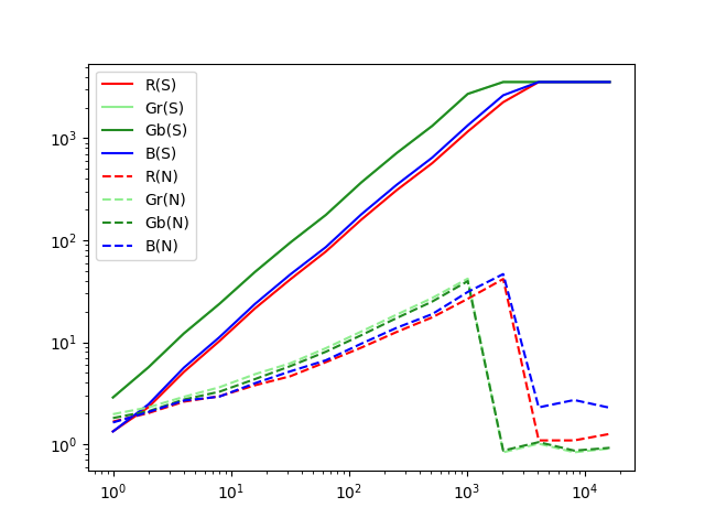
执行这段代码后,将会显示图表。
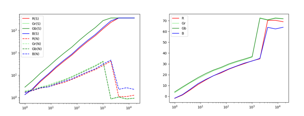
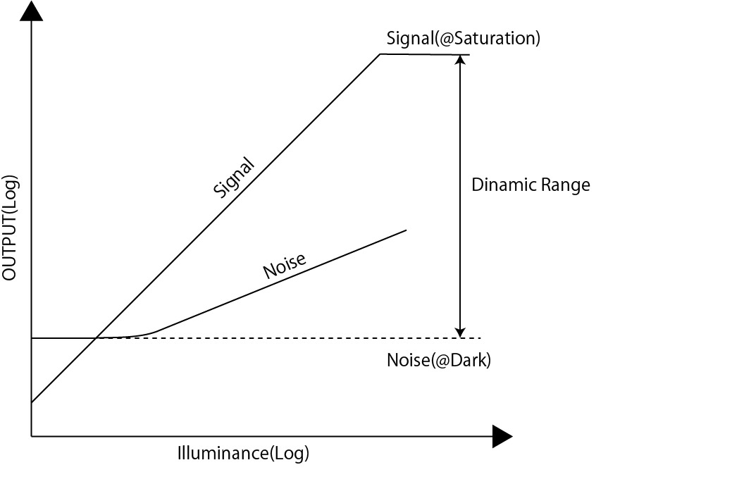
左侧的图表展示了信号和噪声的光量响应特性,右侧则显示了信噪比的特性。从这些结果对 IMX503 进行初步分析,可以得出:
- 显然,信号与光量成正比。
- 噪声大约与信号的平方根成正比。
- 信噪比最大约为 35dB。
- 动态范围约为 70dB。
我们可以得出以上结论!关于动态范围的定义,请查看以下文章。
因此,我对身边的图像传感器进行了简单的分析。这种方法不仅适用于 iPhone,也适用于所有相机,大家可以尝试一下!

コメント