Do you ever take photos with your smartphone? I do from time to time. It’s been a while since smartphones came into the world, and the camera technology has evolved significantly. Nowadays, smartphones can take pictures so beautifully that you might think you no longer need a DSLR. (Though there’s still quite a difference in low-light conditions…)
With that said, I’d like to analyze the performance of the image sensors used in these smartphones!
Image Sensor Used in iPhone
I have an iPhone 12, so the image sensor I’ll be analyzing is the one used in the iPhone 12.
First, I started investigating the image sensor used in the iPhone 12. After doing some research, I found a website that provided useful information. According to this source, the wide-angle camera of the iPhone 12 uses a Sony-made image sensor called the IMX503.
Curious about what kind of sensor the IMX503 is, I looked it up, but I couldn’t find a datasheet no matter how much I searched. It seems that this sensor is not a commercially available product but is likely developed exclusively for Apple.
Image Sensor Measurement Method
Now, let’s get to the main topic: the image sensor analysis method. This time, we will check the sensor’s output response and noise performance. Here’s what you’ll need:
- iPhone (with a camera that can capture Raw images)
- ND filter (15 stops)
- A flat light source
- A dark space
- PC (with Python)
In order to analyze the image sensor, you need to capture Raw images. iPhone users cannot obtain Raw images using the standard camera app. If you want to capture Raw images on an iPhone, try using this app (Simple Raw Camera). The Raw format will be in DNG files.
Make sure to use a flat light source if possible. If you’re a tech enthusiast and happen to own an integrating sphere, that works too. If you don’t have access to a flat light source, you can maximize the brightness of your PC monitor and set it to display solid white.
The ND filter is, of course, used to reduce the amount of light. If you don’t have an ND filter, you can adjust the light levels by changing the shutter speed (though this may alter the noise characteristics).
This is the most important part: always perform the measurements in a completely dark space. This is to ensure linearity near the dark levels.
From here, we’ll move on to the actual measurement process.
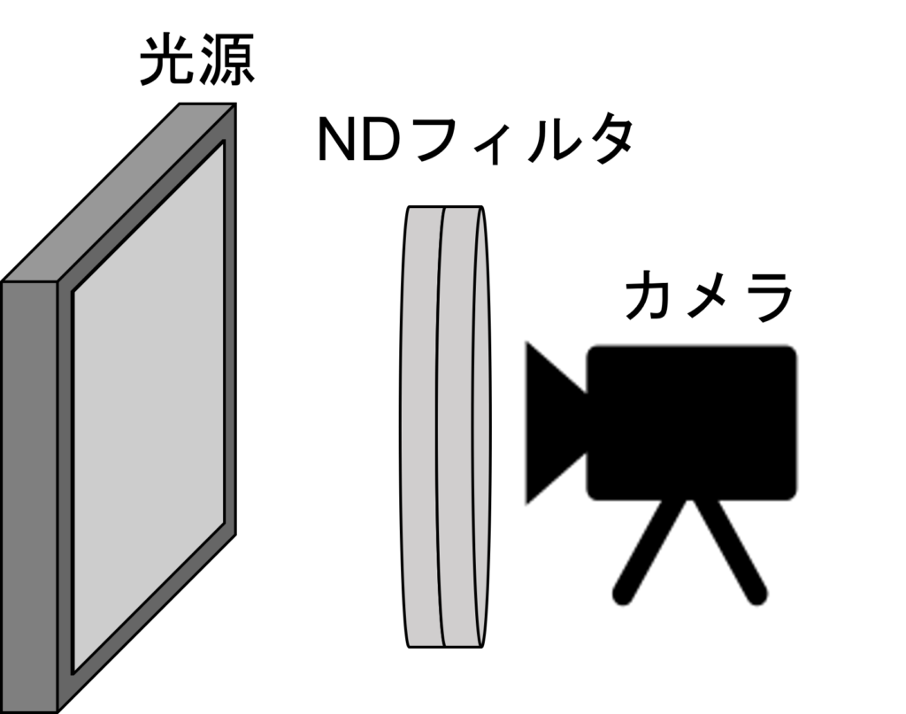
- Fix the position of the light source and the camera (at a distance where the entire ND filter can fit).
- Set the light source to be bright enough so that the camera saturates without the ND filter. If it doesn’t reach saturation, try increasing the shutter speed.。
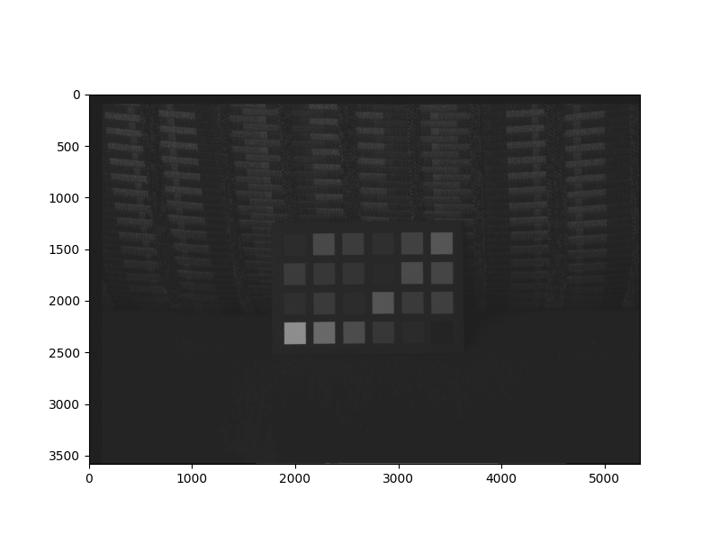
- Take a picture of the light source. Start from the brightest setting, and reduce the light intensity by half each time, repeating the process. You can either insert ND filters or adjust the shutter speed to reduce the light.
- Once you’ve captured images from saturation to a sufficiently dim state, the data collection is complete.
One important note: do not change the distance between the light source and the camera. If you move the light source further away, the brightness will obviously decrease. The setup looks something like this.
Raw Data Analysis
First, Raw images captured by iPhones or DSLRs are specific to each manufacturer’s format. So, make sure to convert them to a standard Raw format before starting the analysis.
We will now analyze the data we have obtained. For this analysis, we will be using Python.
The library we’ll be using this time is as follows:
import numpy as np
import matplotlib.pyplot as plt
import math
Here’s the overall flow of the code. It’s a bit long, but please stick with me until the end.
- Raw image loading settings
- Numpy array settings for image processing
- Settings for handling multiple Raw images
- Dark subtraction (528 in this case)
- Signal, noise, and SNR (Signal-to-Noise Ratio) calculation
- Graph display
That’s the general flow. Below is the actual code.
import numpy as np
import matplotlib.pyplot as plt
import math

#***********************************
#1. Image Settings
#***********************************
width = 4032
height = 3024
width_roi = 100
height_roi = 100
image_num = 15
bit = 12
dark = 528

half_width = int(width / 2)
half_height = int(height / 2)
half_width_roi = int(width_roi / 2)
half_height_roi = int(height_roi / 2)

#***********************************
#2. Array Creation
#***********************************
img_roi = np.empty((height_roi, width_roi), dtype=np.uint16)  # Empty array
img_s = np.empty((4, image_num), dtype=np.float32)
img_n = np.empty((4, image_num), dtype=np.float32)
img_sn = np.empty((4, image_num), dtype=np.float32)
rgb = np.array(range(4))  # For RGB distribution
rgb_det = rgb.reshape((2, 2))  # For RGB distribution
img_roi_r = np.empty((half_height_roi, half_width_roi), dtype=np.uint16)
img_roi_gr = np.empty((half_height_roi, half_width_roi), dtype=np.uint16)
img_roi_gb = np.empty((half_height_roi, half_width_roi), dtype=np.uint16)
img_roi_b = np.empty((half_height_roi, half_width_roi), dtype=np.uint16)
x_axis = np.empty((1, image_num), dtype=np.uint16)

#***********************************
#3. Processing Multiple Raw Images
#***********************************
for i in range(image_num):
    x_axis[0][i] = 2 ** i
    rawpath = "DNG_4032x3024_dark=528_12bit_lin" + str(i) + ".raw"  # Raw image name
    #***********************************
    # Open raw image
    #***********************************
    fd = open(rawpath, 'rb')
    f = np.fromfile(fd, dtype=np.uint16, count=height * width)
    img = f.reshape((height, width))
    fd.close()

    #***********************************
    # Extract ROI
    #***********************************
    width_roi_start = int((width - width_roi) / 2)
    height_roi_start = int((height - height_roi) / 2)
    for x in range(width_roi_start, width_roi_start + width_roi):
        for y in range(height_roi_start, height_roi_start + height_roi):
            img_roi[y - height_roi_start][x - width_roi_start] = img[y][x]

    #***********************************
    # Dark subtraction
    #***********************************
    for x in range(width_roi):
        for y in range(height_roi):
            if img_roi[y][x] > dark:
                img_roi[y][x] = img_roi[y][x] - dark
            elif img_roi[y][x] <= dark:
                img_roi[y][x] = 0

    #***********************************
    # SN Calculation
    #***********************************
    for x in range(width_roi):
        for y in range(height_roi):
            color = rgb_det[y % 2][x % 2]
            if color == 0:  # R
                y_r = int(y / 2)
                x_r = int(x / 2)
                img_roi_r[y_r][x_r] = img_roi[y][x]
            elif color == 1:  # Gr
                y_gr = int(y / 2)
                x_gr = int((x - 1) / 2)
                img_roi_gr[y_gr][x_gr] = img_roi[y][x]
            elif color == 2:  # Gb
                y_gb = int((y - 1) / 2)
                x_gb = int(x / 2)
                img_roi_gb[y_gb][x_gb] = img_roi[y][x]
            else:  # B
                y_gb = int((y - 1) / 2)
                x_gb = int((x - 1) / 2)
                img_roi_b[y_gb][x_gb] = img_roi[y][x]

    # Signal
    img_s[0][i] = np.mean(img_roi_r)
    img_s[1][i] = np.mean(img_roi_gr)
    img_s[2][i] = np.mean(img_roi_gb)
    img_s[3][i] = np.mean(img_roi_b)

    # Noise
    img_n[0][i] = np.std(img_roi_r)
    img_n[1][i] = np.std(img_roi_gr)
    img_n[2][i] = np.std(img_roi_gb)
    img_n[3][i] = np.std(img_roi_b)

    # SNR
    img_sn[0][i] = 20 * (math.log10(img_s[0][i] / img_n[0][i]))
    img_sn[1][i] = 20 * (math.log10(img_s[1][i] / img_n[1][i]))
    img_sn[2][i] = 20 * (math.log10(img_s[2][i] / img_n[2][i]))
    img_sn[3][i] = 20 * (math.log10(img_s[3][i] / img_n[3][i]))

# Display Graphs
fig1 = plt.figure()
ax1 = fig1.add_subplot(111)
ax1.plot(x_axis[0, :], img_sn[0, :], label="R", color="r")
ax1.plot(x_axis[0, :], img_sn[1, :], label="Gr", color="lightgreen")
ax1.plot(x_axis[0, :], img_sn[2, :], label="Gb", color="forestgreen")
ax1.plot(x_axis[0, :], img_sn[3, :], label="B", color="b")
ax1.set_xscale("log")  # Logarithmic axis
ax1.legend()

fig2 = plt.figure()
ax2 = fig2.add_subplot(111)
ax2.plot(x_axis[0, :], img_s[0, :], label="R", color="r")
ax2.plot(x_axis[0, :], img_s[1, :], label="Gr", color="lightgreen")
ax2.plot(x_axis[0, :], img_s[2, :], label="Gb", color="forestgreen")
ax2.plot(x_axis[0, :], img_s[3, :], label="B", color="b")
ax2.plot(x_axis[0, :], img_n[0, :], linestyle="--", label="R", color="r")
ax2.plot(x_axis[0, :], img_n[1, :], linestyle="--", label="Gr", color="lightgreen")
ax2.plot(x_axis[0, :], img_n[2, :], linestyle="--", label="Gb", color="forestgreen")
ax2.plot(x_axis[0, :], img_n[3, :], linestyle="--", label="B", color="b")
ax2.set_xscale("log")  # Logarithmic axis
ax2.set_yscale("log")  # Logarithmic axis
ax2.legend()

plt.show()
When you run this code, the graphs will be displayed.
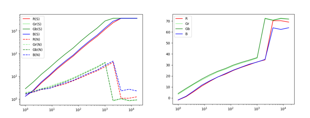
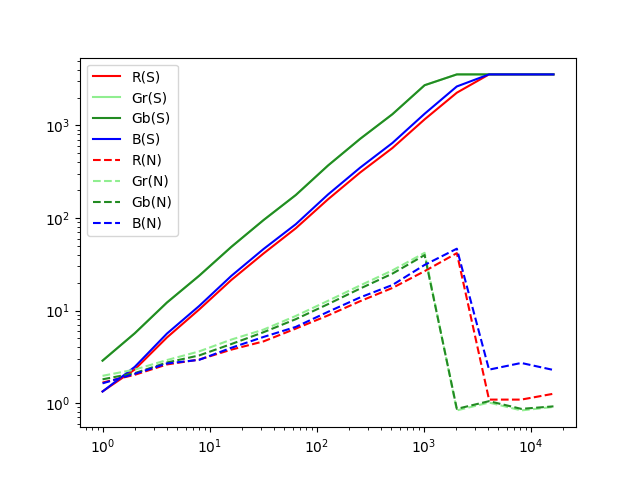
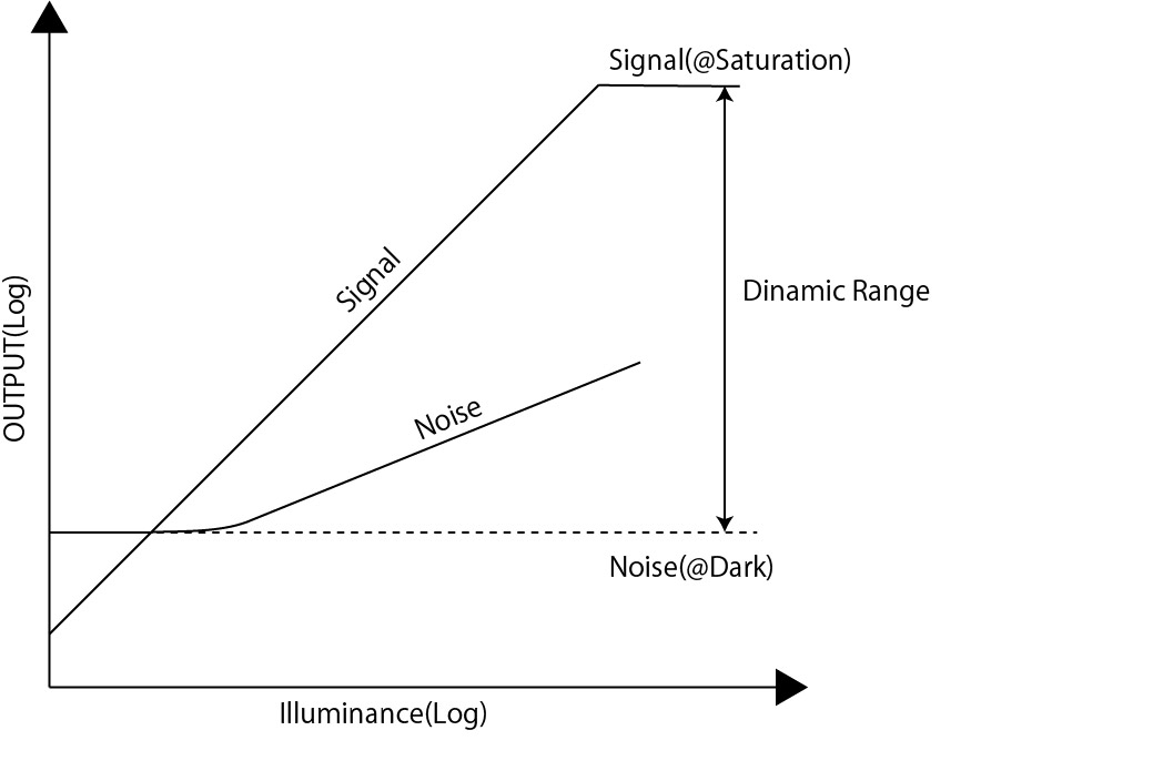
The graph on the left shows the response characteristics of signal and noise relative to light intensity. The one on the right shows the SNR (Signal-to-Noise Ratio) characteristics.
From these results, a rough analysis of the IMX503 shows that…
- As expected, the signal is proportional to the light intensity.
- The noise is approximately proportional to the square root of the signal.
- The SNR (Signal-to-Noise Ratio) reaches a maximum of about 35dB
- The dynamic range is approximately 70dB.
We have confirmed these results! For the definition of dynamic range, please refer to the article below.
So, this was a simple analysis of the image sensor you can find in everyday devices. This method can be used not only for iPhones but for any camera, so feel free to give it a try!


コメント