大家會用手機拍照嗎?我偶爾會拍。自從手機誕生以來,已經過了一段時間,攝影技術也進步了很多。現在,拍出來的照片幾乎跟單眼相機一樣漂亮,讓人覺得或許不需要單眼相機了。(當然在暗處的表現還是有差別的……)
接下來,我想來解析一下這些智慧型手機裡使用的影像感測器的實力吧!
iPhone 所使用的影像感測器
我手上的手機是 iPhone 12 標準版,所以這次要解析的是 iPhone 12 所使用的影像感測器。
首先,我調查了 iPhone 12 使用的影像感測器。在搜尋了很多資料後,我找到了這樣的一個網站。根據該網站的資訊,iPhone 12 的廣角鏡頭使用的是 Sony 製的 IMX503 影像感測器。
我很好奇 IMX503 是什麼樣的感測器,於是進一步查找,但無論怎麼找都沒有找到資料表。我推測這應該不是市面上的產品,而是專為 Apple 開發的感測器。
影像感測器的測量方法
那麼,接下來進入正題,來講解影像感測器的解析方法。這次我們將確認感測器的輸出響應和噪音性能。所需準備的東西如下:
- iPhone(能拍攝 Raw 圖像的相機)
- 15 段 ND 濾鏡
- 平坦的光源
- 黑暗的空間
- PC(Python)
在分析影像感測器時,必須取得 Raw 圖像。iPhone 使用者無法通過普通的相機應用程式來拍攝 Raw 圖像。若要在 iPhone 上取得 Raw 圖像,請嘗試使用這個應用程式(Simple Raw Camera)。Raw 圖像的格式是 DNG 檔案。
光源請盡量使用平坦的光源。如果你是擁有積分球的技術迷,那麼可以使用積分球。如果沒有平坦的光源,可以將 PC 的螢幕亮度調至最大並設為全白,這也是一種選擇。
ND 濾鏡當然是用來減少光量的。如果無法準備 ND 濾鏡,可以嘗試調整快門速度來改變光量。(不過,這可能會改變噪音特性。)
這裡最重要的一點是,一定要在完全黑暗的空間中進行測量。這是為了確保暗部的線性特性。
接下來是實際的測量方法。
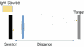
- 將光源和相機的位置固定。(距離應能完全容納 ND 濾鏡)
- 請將光源調亮,直到相機在沒有 ND 濾鏡的情況下達到飽和。如果光源無法達到飽和,請嘗試延長快門速度。
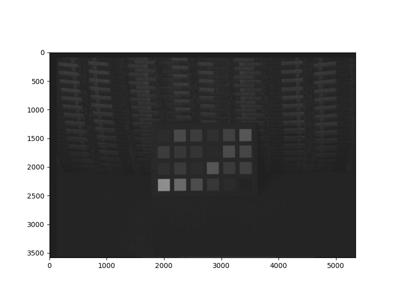
- 拍攝光源。從最亮的狀態開始,每次將光量減半,重複拍攝。要減少光量,可以加入 ND 濾鏡或調整快門速度。
- 當你從飽和狀態拍攝到足夠暗的狀態後,數據採集就完成了。
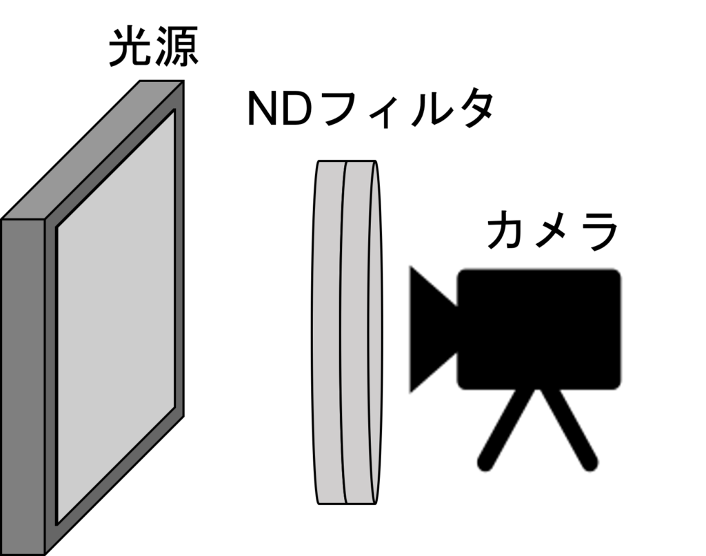
注意事項是,請勿改變光源與相機之間的距離。如果將光源移遠,光量自然會變暗。配置的示意圖如下所示。
Raw 資料的解析
首先,iPhone 或 DSLR 所拍攝的 Raw 圖像各廠商都有其專屬格式,因此請先將其轉換為通用的 Raw 格式後,再進行解析。
接下來,我們將對取得的數據進行解析。這次我們將使用 Python 來進行解析。
以下是我們將使用的庫:
import numpy as np
import matplotlib.pyplot as plt
import math
這是整個程式碼的流程。雖然有點長,但請耐心看完。
- Raw 圖像讀取設定
- 用於圖像處理的 Numpy 陣列設定
- 處理多張 Raw 圖像的設定
- 減去暗電流(這次設定為 528)
- 計算信號、噪音和 SN 比
- 顯示圖表
以上是整體流程。以下是實際的程式碼。
import numpy as np
import matplotlib.pyplot as plt
import math

#***********************************
#1. 圖像設定
#***********************************
width=4032
height=3024
width_roi = 100
height_roi = 100
image_num = 15
bit = 12
dark = 528 #

half_width = int(width/2)
half_height = int(height/2)
half_width_roi = int(width_roi/2)
half_height_roi = int(height_roi/2)

#***********************************
#2. 各種陣列創建
#***********************************
img_roi=np.empty((height_roi, width_roi),dtype = np.uint16) #空陣列
img_s = np.empty((4,image_num),dtype = np.float32)
img_n = np.empty((4,image_num),dtype = np.float32)
img_sn = np.empty((4,image_num),dtype = np.float32)
rgb = np.array(range(4)) #用於 RGB 分配
rgb_det = rgb.reshape((2,2)) #用於 RGB 分配
img_roi_r=np.empty((half_height_roi, half_width_roi),dtype = np.uint16)
img_roi_gr=np.empty((half_height_roi, half_width_roi),dtype = np.uint16)
img_roi_gb=np.empty((half_height_roi, half_width_roi),dtype = np.uint16)
img_roi_b=np.empty((half_height_roi, half_width_roi),dtype = np.uint16)
x_axis = np.empty((1,image_num),dtype = np.uint16)

#***********************************
#3. 多張 Raw 處理
#***********************************
for i in range(image_num):
    x_axis[0][i] = 2**i
    rawpath = "DNG_4032x3024_dark=528_12bit_lin"+str(i)+".raw" #Raw 圖像的名稱
    #***********************************
    # 開啟 Raw 圖像
    #***********************************
    fd = open(rawpath, 'rb')
    f = np.fromfile(fd, dtype=np.uint16, count=height*width)
    img = f.reshape((height,width))
    fd.close()

    #***********************************
    # 提取 ROI
    #***********************************
    width_roi_start = int((width-width_roi)/2)
    height_roi_start = int((height-height_roi)/2)
    for x in range(width_roi_start,width_roi_start+width_roi):
        for y in range(height_roi_start,height_roi_start+height_roi):
            img_roi[y-height_roi_start][x-width_roi_start] = img[y][x]

    #***********************************
    # 去除暗電流
    #***********************************
    for x in range(width_roi):
        for y in range(height_roi):
            if img_roi[y][x] > dark:
                img_roi[y][x] = img_roi[y][x]-dark
            elif img_roi[y][x] <= dark:
                img_roi[y][x] = 0

    #***********************************
    # SN 計算
    #***********************************
    for x in range(width_roi):
        for y in range(height_roi):
            color = rgb_det[y % 2][x % 2]
            if color == 0: #R
                y_r = int(y/2)
                x_r = int(x/2)
                img_roi_r[y_r][x_r] = img_roi[y][x]
            elif color == 1: #Gr
                y_gr = int(y/2)
                x_gr = int((x-1)/2)
                img_roi_gr[y_gr][x_gr] = img_roi[y][x]
            elif color == 2: #Gb
                y_gb = int((y-1)/2)
                x_gb = int(x/2)
                img_roi_gb[y_gb][x_gb] = img_roi[y][x]
            else: #B
                y_gb = int((y-1)/2)
                x_gb = int((x-1)/2)
                img_roi_b[y_gb][x_gb] = img_roi[y][x]
    # 信號
    img_s[0][i] = np.mean(img_roi_r)
    img_s[1][i] = np.mean(img_roi_gr)
    img_s[2][i] = np.mean(img_roi_gb)
    img_s[3][i] = np.mean(img_roi_b)
    # 噪音
    img_n[0][i] = np.std(img_roi_r)
    img_n[1][i] = np.std(img_roi_gr)
    img_n[2][i] = np.std(img_roi_gb)
    img_n[3][i] = np.std(img_roi_b)
    # SN 比
    img_sn[0][i] = 20*(math.log10(img_s[0][i]/img_n[0][i]))
    img_sn[1][i] = 20*(math.log10(img_s[1][i]/img_n[1][i]))
    img_sn[2][i] = 20*(math.log10(img_s[2][i]/img_n[2][i]))
    img_sn[3][i] = 20*(math.log10(img_s[3][i]/img_n[3][i]))

# 顯示圖表
fig1 = plt.figure()
ax1 = fig1.add_subplot(111)
ax1.plot(x_axis[0,:], img_sn[0,:],label = "R",color = "r")
ax1.plot(x_axis[0,:], img_sn[1,:],label = "Gr",color = "lightgreen")
ax1.plot(x_axis[0,:], img_sn[2,:],label = "Gb",color = "forestgreen")
ax1.plot(x_axis[0,:], img_sn[3,:],label = "B",color = "b")
ax1.set_xscale("log") # 軸對數化
ax1.legend()

fig2 = plt.figure()
ax2 = fig2.add_subplot(111)
ax2.plot(x_axis[0,:], img_s[0,:],label = "R",color = "r")
ax2.plot(x_axis[0,:], img_s[1,:],label = "Gr",color = "lightgreen")
ax2.plot(x_axis[0,:], img_s[2,:],label = "Gb",color = "forestgreen")
ax2.plot(x_axis[0,:], img_s[3,:],label = "B",color = "b")
ax2.plot(x_axis[0,:], img_n[0,:],linestyle="--",label = "R",color = "r")
ax2.plot(x_axis[0,:], img_n[1,:],linestyle="--",label = "Gr",color = "lightgreen")
ax2.plot(x_axis[0,:], img_n[2,:],linestyle="--",label = "Gb",color = "forestgreen")
ax2.plot(x_axis[0,:], img_n[3,:],linestyle="--",label = "B",color = "b")
ax2.set_xscale("log") # 軸對數化
ax2.set_yscale("log") # 軸對數化
ax2.legend()

plt.show()
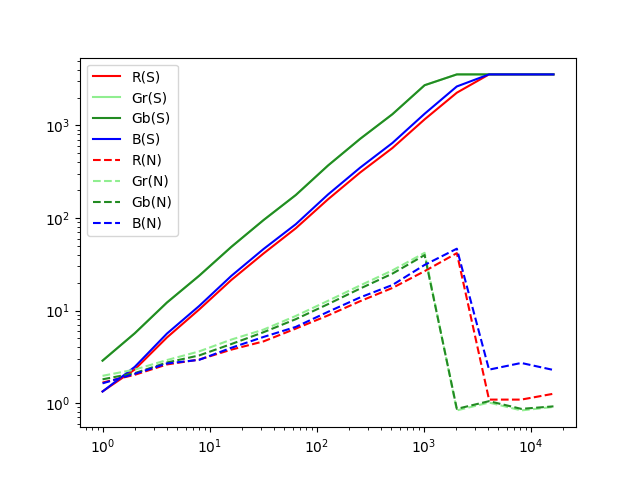
執行此程式後,將會顯示圖表。
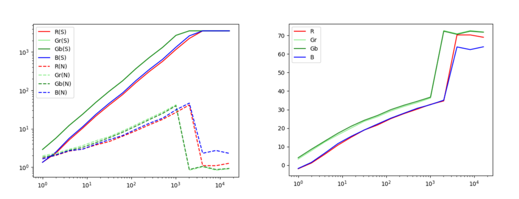
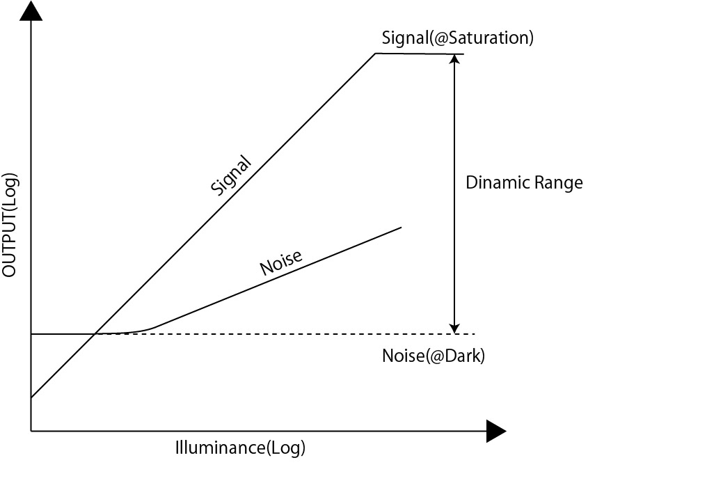
左邊的圖表顯示的是信號和噪音相對光量的響應特性,右邊的是 SN 比的特性。
根據這些結果,對 IMX503 的大致分析如下:
- 信號當然是與光量成正比的。
- 噪音大約與信號的平方根成正比。
- SN 比最大約為 35dB。
- 動態範圍約為 70dB。
這就是我們所得到的結果!動態範圍的定義請參考以下的文章。
因此,我對身邊的影像感測器進行了簡單的解析。這是一種不僅適用於 iPhone,而是適用於所有相機的方法,大家不妨試試看!

コメント